Example
This example demonstrates a simple RSI-based strategy on QQQ data.
import oequant as oq
import pandas_ta as ta
from bokeh.io import output_notebook

# Required for Bokeh plots in notebooks
output_notebook()

# 1. Get Data
ticker = "QQQ"
start_date = "2010-01-01"
end_date = "2025-05-01"
data = oq.get_data(ticker, start=start_date, end=end_date)

# 2. Add Indicator & Signals
# Calculate RSI_3
data.ta.rsi(length=3, append=True, col_names=('rsi_3',))
# Calculate exit signal: close > high.shift()
data['exit_signal'] = data['close'] > data['high'].shift(1)
# Entry signal: rsi_3 < 20 (will be passed as an expression)
entry_expression = "rsi_3 < 20"
data.dropna(inplace=True) # Drop NaNs from indicator calculation

# 3. Run Backtest
results = oq.backtest(
    data=data,
    entry_column=entry_expression,
    exit_column='exit_signal',
    fee_frac=0.001,
    capital=100_000
)

# 4. Show Report and Plot
results.report(show_plot=True, plot_args={
    'indicators_other': ['rsi_3'],
    'per_indicator_plot_height': 160,
    'plot_theme': 'dark'
})
Sample Output
--- Backtest Report ---
Start Date:             2010-01-04
End Date:               2025-04-30
Duration:               5595 days 00:00:00
Initial Capital:        100,000.00
Final Equity:           211,555.28
Benchmark Final Equity: 1,174,411.72

--- Performance Metrics ---
|                    |   Strategy |   Benchmark |
|====================|============|=============|
|           CAGR (%) |      5.02% |      17.47% |
|      Avg Trade (%) |      0.47% |   1,074.41% |
|       Sharpe Ratio |     0.5031 |      0.8771 |
|      Sortino Ratio |     0.3253 |      1.1264 |
| Time in Market (%) |     15.93% |      99.97% |
|   Max Drawdown (%) |    -16.14% |     -35.12% |
|      CAGR / Max DD |     0.3111 |      0.4975 |
|     Serenity Ratio |     4.3518 |      3.1370 |
|       Total Trades |   169.0000 |      1.0000 |
|       Win Rate (%) |     69.23% |     100.00% |
|      Loss Rate (%) |     30.77% |       0.00% |
|  Avg Win Trade (%) |      1.52% |   1,074.41% |
| Avg Loss Trade (%) |     -1.90% |       0.00% |
|      Profit Factor |     1.7373 |         inf |
|      Avg Bars Held |     3.6331 |  3,854.0000 |
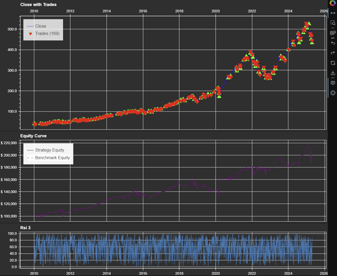
An interactive plot showing the price, trades, equity curve, benchmark, and RSI indicator would also be displayed: